Bidiagonal matrix

In mathematics, a bidiagonal matrix is a banded matrix with non-zero entries along the main diagonal and either the diagonal above or the diagonal below. This means there are exactly two non-zero diagonals in the matrix.

When the diagonal above the main diagonal has the non-zero entries the matrix is upper bidiagonal. When the diagonal below the main diagonal has the non-zero entries the matrix is lower bidiagonal.

For example, the following matrix is upper bidiagonal: $${\begin{pmatrix}1&4&0&0\\0&4&1&0\\0&0&3&4\\0&0&0&3\\\end{pmatrix}}$$

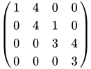
and the following matrix is lower bidiagonal:

$${\begin{pmatrix}1&0&0&0\\2&4&0&0\\0&3&3&0\\0&0&4&3\\\end{pmatrix}}.$$

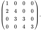
The eigenvalues of a bidiagonal matrix (of either type) are given by the entries of the diagonal.

For a square bidiagonal matrix B, the determinant is simply the product of its diagonal elements:

$\det(B)=\prod _{i=1}^{n}b_{ii}$

Additionally, the inverse of a nonsingular upper bidiagonal matrix B is an upper triangular matrix whose entries can be computed explicitly without solving full systems of linear equations.

Usage

One variant of the QR algorithm starts with reducing a general matrix into a bidiagonal one, and the singular value decomposition (SVD) uses this method as well.

Singular Value Decomposition

Reducing a matrix to bidiagonal form is a standard first step in the Golub-Kahan algorithm for computing the SVD. Because Householder reflections or Given rotations can reduce a dense $m\times n$ matrix to an equivalent bidiagonal matrix in ${\mathcal {O}}(m\times n^{2})$ operations, working with the bidiagonal structure drastically reduces the computational cost of subsequent iterative SVD and QR steps.

High Relative Accuracy in Ill-Conditioned Systems

For general dense matrices, standard numerical algorithms compute singular values with an absolute error bound proportional to the largest singular value. If the matrix is ill-conditioned, this can result in a total loss of precision for the smallest singular values.

Because of this, specialized algorithms such as the zero-shift bidiagonal QR algorithm or the differential qd (dqd) algorithm developed by James Demmel and William Kahan can compute all the singular values of a bidiagonal matrix to high relative accuracy, regardless of the matrix's condition number.

See also

• List of matrices
• Singular value decomposition
• Lanczos algorithm
• LAPACK
• Hessenberg form — The Hessenberg form is similar, but has more non-zero diagonal lines than 2.

References

• Stewart, G.W. (2001). Eigensystems. Matrix Algorithms. Vol. 2. Society for Industrial and Applied Mathematics. ISBN 0-89871-503-2.

External links

• High performance algorithms for reduction to condensed (Hessenberg, tridiagonal, bidiagonal) form

References

[edit]- Stewart, G.W. (2001). Eigensystems. Matrix Algorithms. Vol. 2. Society for Industrial and Applied Mathematics. ISBN 0-89871-503-2.
- ↑ Anatolyevich, Bochkanov Sergey (2010-12-11). "Matrix operations and decompositions — Other operations on general matrices — SVD decomposition". ALGLIB User Guide, ALGLIB Project. Accessed: 2010-12-11. (Archived by WebCite at)
- ↑ "Calculating the Singular Values and Pseudo-Inverse of a Matrix | SIAM Journal on Numerical Analysis". Journal of the Society for Industrial and Applied Mathematics, Series B: Numerical Analysis. doi:10.1137/0702016.
- ↑ Golub, Gene H.; Van Loan, Charles F. (2013). "Section 8.6.1: Properties and Perturbation Theory". Matrix Computations (4th ed.). Johns Hopkins University Press. pp. 486–487. ISBN 978-1421407944.
- ↑ Demmel, James; Kahan, William (1990). "Accurate Singular Values of Bidiagonal Matrices". SIAM Journal on Scientific and Statistical Computing. 11 (5): 873–912. doi:10.1137/0911052.